The introduction of deep convolutional neural networks (CNNs) has dramatically improved image recognition capabilities. Among the seminal architectures, the VGG Architecture, proposed by Karen Simonyan and Andrew Zisserman in 2014, was a breakthrough. It demonstrated the effectiveness of deep, simple, and uniform layer structures in achieving state-of-the-art performance on the ImageNet dataset.

VGG Architecture Overview

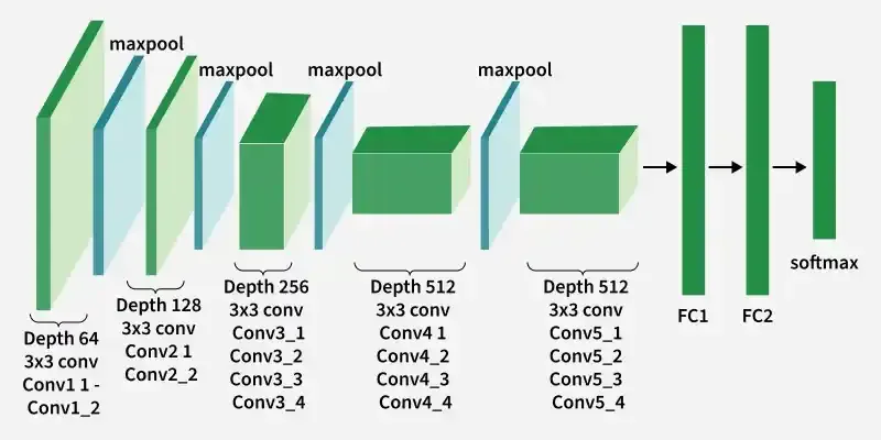
The hallmark of VGG lies in its simplicity and depth. The architecture systematically increases the depth of the network by stacking small convolutional filters (3×3 kernels) while maintaining a consistent structure across layers. This design enables the network to learn hierarchical features effectively, from simple edges in shallow layers to complex patterns in deeper ones.

Design Principles

1. Uniform Convolutional Layers:
   • VGG exclusively uses 3×3 filters with a stride of 1 and padding of 1.
   • These filters minimize computational complexity while ensuring that each convolutional layer extracts features within a small receptive field.
2. Max-Pooling for Down-Sampling:
   • 2×2 max-pooling layers with a stride of 2 follow blocks of convolutional layers.
   • This down-sampling strategy reduces spatial dimensions progressively, allowing the network to focus on high-level features.
3. Deep Stack of Convolutional Blocks:
   • Each convolutional block contains multiple convolutional layers followed by a pooling layer.
   • The number of filters in convolutional layers doubles after each pooling operation (e.g., 64, 128, 256, 512).
4. Fully Connected Layers:
   • After convolutional and pooling layers, the spatial features are flattened and passed through three fully connected layers, ending with a softmax layer for classification.

VGG-16 Architecture & Training Overview

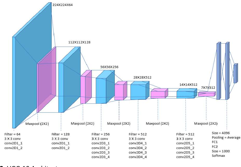
VGG-16 (developed by the Visual Geometry Group at Oxford) is a landmark Convolutional Neural Network (CNN) architecture designed for image classification. Its primary hallmark is its simplicity and uniform design, relying strictly on $3 \times 3$ convolutions with stride 1 and $2 \times 2$ max-pooling with stride 2 throughout the entire feature extractor.

Key Specifications

• Total Weight Layers: 16 (13 Convolutional layers + 3 Fully Connected layers).
• Total Parameters: ~138 Million (over 100M of which reside in the first fully connected layer).
• Input Dimension: $224 \times 224 \times 3$ (RGB).
• Model Size: ~528 MB.

VGG-16 Architecture Breakdown

Each of the 5 convolutional blocks ends with a $2 \times 2$ Max-Pooling layer (stride = 2), which halves the spatial height and width ($H \times W$) while doubling feature channels in subsequent blocks.

Stage / Block	Layer Type	Kernel Size / Stride	Filters / Neurons	Spatial Output Shape
Input	Image Input	—	3 channels	$224 \times 224 \times 3$
Block 1	2 $\times$ Conv3D + MaxPool	$3 \times 3$, stride 1	64	$112 \times 112 \times 64$
Block 2	2 $\times$ Conv3D + MaxPool	$3 \times 3$, stride 1	128	$56 \times 56 \times 128$
Block 3	3 $\times$ Conv3D + MaxPool	$3 \times 3$, stride 1	256	$28 \times 28 \times 256$
Block 4	3 $\times$ Conv3D + MaxPool	$3 \times 3$, stride 1	512	$14 \times 14 \times 512$
Block 5	3 $\times$ Conv3D + MaxPool	$3 \times 3$, stride 1	512	$7 \times 7 \times 512$
FC 1	Fully Connected + Dropout	$7 \times 7$ Flatten	4,096	$1 \times 1 \times 4096$
FC 2	Fully Connected + Dropout	Dense	4,096	$1 \times 1 \times 4096$
FC 3 (Output)	Fully Connected + Softmax	Dense	1,000	$1 \times 1 \times 1000$

Key Architectural Design Innovations

1. Stacked Small Kernels ($3 \times 3$):
   • Stacking two $3 \times 3$ conv layers has an effective receptive field of a single $5 \times 5$ conv layer.
   • Stacking three $3 \times 3$ conv layers equals a $7 \times 7$ receptive field.
   • Advantage: Stacking smaller kernels incorporates non-linear activation functions (ReLU) after every layer while significantly reducing the parameter count compared to larger kernels.

Read more blog: VGG and LeNet-5 Architectures: Key Differences and Real-World Applications

1. Symmetric Downsampling:
   • Spatial dimensions are halved strictly by Max-Pooling ($2 \times 2$, stride 2), while feature depth doubles at each block transition (64 $\rightarrow$ 128 $\rightarrow$ 256 $\rightarrow$ 512).

Training Insights & Optimization Strategy

1. Weight Initialization

• Original Paper: Initial shallow configurations (e.g., VGG-11) were trained with zero-mean Gaussian initialization ($\sigma = 0.01$). Deeper nets like VGG-16 were initialized using pre-trained weights from the shallower layers.
• Modern Practice: He (Kaiming) Initialization or Xavier (Glorot) Initialization is used to avoid vanishing/exploding gradients when training from scratch without multi-stage pre-training.

2. Activation Function & Regularization

• ReLU (Rectified Linear Unit): Applied after every convolutional and fully connected layer to introduce non-linearity, mitigate vanishing gradients, and accelerate convergence.
• Dropout: Applied to the first two fully connected layers (FC1 and FC2) with a probability rate of $0.5$ to prevent over-fitting.
• Batch Normalization (VGG-16_BN): Introduced in modern frameworks (e.g., PyTorch/TensorFlow) between the Convolutional layer and ReLU to normalize activations, stabilize training, and allow higher learning rates.

3. Optimization Parameters

• Optimizer: Stochastic Gradient Descent (SGD) with momentum ($0.9$).
• Weight Decay: $L_2$ regularization with a weight decay multiplier of $5 \times 10^{-4}$.
• Learning Rate Schedule: Initial learning rate of $0.01$, reduced by a factor of 10 whenever validation set accuracy plateaus.

4. Objective Function

• Categorical Cross-Entropy Loss: Used alongside a final 1,000-class Softmax activation layer to measure discrepancies between class probability distribution and ground-truth one-hot labels.

Why Depth Matters

VGG demonstrated that increasing the network’s depth allows it to learn hierarchical feature representations more effectively.

1. Feature Hierarchy:
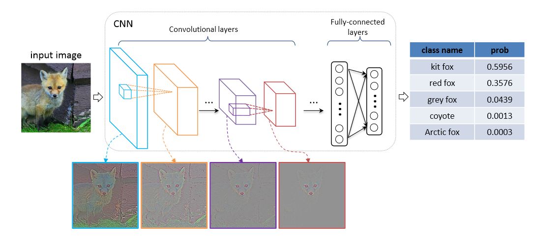
   • Early layers capture low-level features like edges and textures.
   • Intermediate layers focus on shapes and objects.
   • Deep layers identify semantic concepts like faces or animals.
2. Receptive Field Expansion:
   • The depth allows small kernels (3×3) to incrementally expand the receptive field. For example, stacking three 3×3 filters covers the same area as a 7×7 kernel but retains more parameters to model complex patterns.

Computational Complexity

The key limitation of VGG lies in its computational demand:

1. Parameter Count:
   • VGG-16 has 138 million parameters, leading to large memory requirements and slow inference on resource-constrained systems.
2. Redundancy:
   • The fully connected layers alone account for a significant portion of parameters, introducing redundancy in feature representation.
3. Training Time:
   • Due to its depth and high parameter count, training requires powerful hardware (e.g., GPUs) and long periods to converge.

Technical Comparisons with Successors

While VGG revolutionized image recognition, its limitations led to the development of more efficient architectures like ResNet, Inception, and EfficientNet:

1. Residual Connections (ResNet):
   • ResNet mitigates the vanishing gradient problem by introducing skip connections, enabling networks to go even deeper.
2. Multi-Scale Filters (Inception):
   • Inception employs filters of varying sizes in parallel to capture features at multiple scales, reducing redundancy.
3. Compound Scaling (EfficientNet):
   • EfficientNet optimizes network width, depth, and resolution using a compound scaling strategy for higher efficiency.

Implementing VGG-16 with PyTorch

Below is a modular PyTorch implementation of the VGG-16 architecture from scratch. The configuration array VGG16_CONFIG dynamically constructs the 5 convolutional blocks, followed by the fully connected classification head.

import torch
import torch.nn as nn

# Configuration layout for VGG-16:
# Integers represent output filter channels; 'M' represents MaxPool2d (2x2, stride 2)
VGG16_CONFIG = [
    64, 64, 'M',
    128, 128, 'M',
    256, 256, 256, 'M',
    512, 512, 512, 'M',
    512, 512, 512, 'M'
]

class VGG16(nn.Module):
    def __init__(self, in_channels: int = 3, num_classes: int = 1000):
        super(VGG16, self).__init__()
        self.in_channels = in_channels
        self.features = self._create_conv_layers(VGG16_CONFIG)
        
        self.classifier = nn.Sequential(
            nn.Flatten(),
            nn.Linear(512 * 7 * 7, 4096),
            nn.ReLU(inplace=True),
            nn.Dropout(p=0.5),
            nn.Linear(4096, 4096),
            nn.ReLU(inplace=True),
            nn.Dropout(p=0.5),
            nn.Linear(4096, num_classes)
        )

    def forward(self, x: torch.Tensor) -> torch.Tensor:
        x = self.features(x)
        x = self.classifier(x)
        return x

    def _create_conv_layers(self, config: list) -> nn.Sequential:
        layers = []
        in_channels = self.in_channels
        
        for layer in config:
            if isinstance(layer, int):
                out_channels = layer
                layers.extend([
                    nn.Conv2d(in_channels, out_channels, kernel_size=3, stride=1, padding=1),
                    nn.BatchNorm2d(out_channels),  # Modern integration for training stability
                    nn.ReLU(inplace=True)
                ])
                in_channels = out_channels
            elif layer == 'M':
                layers.append(nn.MaxPool2d(kernel_size=2, stride=2))
                
        return nn.Sequential(*layers)

# Quick Shape Verification
if __name__ == "__main__":
    model = VGG16(in_channels=3, num_classes=1000)
    x = torch.randn(2, 3, 224, 224)  # Batch of 2 RGB images
    output = model(x)
    print(f"Output shape: {output.shape}")  # Expected: torch.Size([2, 1000])

Advantages of VGG

• Uniform & Modular Design: By standardizing every convolutional layer to $3 \times 3$ filters with a stride of 1 and padding of 1, VGG established an intuitive design paradigm that proved deeper networks could outperform handcrafted, multi-scale feature extractors.
• Effective Receptive Field Expansion: Stacking three $3 \times 3$ convolutions provides the same receptive field as a single $7 \times 7$ convolution, but incorporates three non-linear activation layers (ReLU) instead of one while using significantly fewer parameters.
• Premier Backbone for Transfer Learning: The hierarchical spatial features learned across VGG’s blocks generalize exceptionally well to downstream tasks. Pre-trained VGG weights remain widely used as feature extractors in object detection backbones (e.g., Faster R-CNN), image segmentation (U-Net feature extraction), and style transfer algorithms (calculating Gram matrix perceptual loss).

Limitations of VGG

• Massive Parameter Memory Footprint: VGG-16 contains ~138 million parameters, occupying over 520 MB of storage space. More than 70% of these parameters reside in the dense fully connected classification layers (FC1 alone accounts for ~102M weights).
• High Computational Cost (FLOPs): Processing a single $224 \times 224$ RGB image requires ~15.5 GFLOPs. This heavy computational burden makes VGG unsuitable for real-time inference on edge devices, mobile chips, or resource-constrained embedded systems.
• Vanishing Gradient Bottleneck: Due to its linear sequence of stacked layers without skip connections, training deeper variants (such as VGG-19) becomes unstable. Modern architectures like ResNet (introducing residual skip connections) and Inception (introducing multi-scale branching) achieved superior accuracy with a fraction of VGG’s parameter footprint and memory usage.

VGG’s Legacy in Modern AI

Though newer architectures have outpaced VGG in efficiency and accuracy, its legacy is undeniable. Here’s how VGG continues to impact the field:

1. Foundation for Transfer Learning: VGG models, pre-trained on ImageNet, are still widely used in various applications. Researchers fine-tune these models to solve domain-specific problems with limited data.
2. Inspiration for Depth-Oriented Architectures: VGG’s success demonstrated the value of depth in CNNs, inspiring architectures like ResNet, DenseNet, and EfficientNet, which build on its principles.
3. Use in Feature Extraction: The hierarchical features learned by VGG are leveraged for non-classification tasks like style transfer and image captioning.

Applications of VGG in Real-World Scenarios

1. Medical Imaging: VGG has been employed to classify X-rays, detect tumors in MRI scans, and identify diseases in histopathology images.
2. Autonomous Vehicles: VGG-based models contribute to object detection systems in self-driving cars, recognizing pedestrians, vehicles, and traffic signs.
3. Facial Recognition: VGG’s feature extraction capabilities are utilized in facial recognition systems for security and authentication.
4. Art and Creativity: VGG underpins applications like neural style transfer, blending the features of an image with artistic styles.

Conclusion

The VGG architecture laid the foundation for deep CNNs by showing that depth, coupled with simplicity, could achieve remarkable results. While its computational demands have been surpassed by modern architectures, VGG’s influence on network design and feature learning remains a cornerstone in computer vision. For practitioners, understanding VGG is essential for mastering the evolution of CNNs and applying deep learning to complex image recognition tasks.

Frequently Ask Question: