


In the realm of statistics, one of the fundamental concepts to grasp is the variability or dispersion within a dataset. Simply put, dispersion measures how spread out or clustered data points are around the central tendency. It is crucial for understanding the distribution of data and making informed decisions in various fields such as finance, economics, psychology, and more.
Understanding Dispersion:
Dispersion refers to the extent to which data points in a dataset deviate from the central value or mean. A dataset with high dispersion indicates that the data points are spread widely apart, while low dispersion suggests that the data points are closely clustered around the mean. Dispersion provides valuable insights into the consistency, stability, and predictability of data. Artificial Intelligence.
Types of Measures of Dispersion
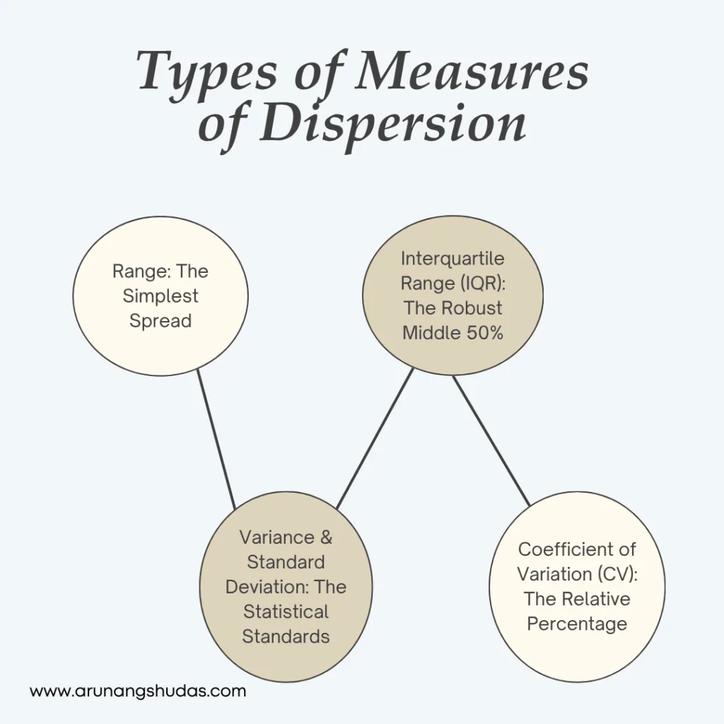
Quantifying the spread of a dataset is essential for understanding data consistency, stability, and predictability. While central tendency metrics (like the mean or median) tell you where the center of your data lies, measures of dispersion reveal how scattered the data points are around that center.
Here are the five most commonly used methods to calculate dispersion, broken down from simplest to most advanced.
1. Range: The Simplest Spread
The range is the most straightforward measurement of dispersion. It calculates the total span of the data from its lowest to highest point.
- The Formula: $\text{Range} = \text{Maximum Value} – \text{Minimum Value}$
- Example: In an exam score dataset where the lowest score is 60 and the highest is 90, the range is 30.
- Pros & Cons: While exceptionally easy to compute as a quick initial indicator, it is highly sensitive to outliers. A single extreme value can drastically skew the results and lead to misleading conclusions.
2. Interquartile Range (IQR): The Robust Middle 50%
The Interquartile Range focuses strictly on the middle portion of your dataset, making it a highly robust measure that successfully mitigates the impact of extreme outliers.
To find the IQR, a dataset is divided into quartiles (four equal parts). The median splits the lower and upper halves, while $Q_1$ marks the 25th percentile and $Q_3$ marks the 75th percentile.
- The Formula: $\text{IQR} = Q_3 – Q_1$
- Example: If a test score dataset has a $Q_1$ of 70 and a $Q_3$ of 85, the IQR is 15. This means the central 50% of your data spans a 15-point intervals.
- Best Used For: Skewed or non-normally distributed data where you want to reliably assess variability around the median without outlier distortion.
Read more blog : Normal Distribution: Comprehensive Guide 2026
3. Variance & Standard Deviation: The Statistical Standards
These two closely related measures are the gold standards in statistical analysis, widely used across finance, economics, and data science.
Variance ($\sigma^2$)
Variance measures the average degree to which each data point deviates from the mean. Because it uses squared differences, it eliminates negative numbers but inflates the unit of measurement.
$$\sigma^2 = \frac{1}{N} \sum_{i=1}^{N} (x_i – \bar{x})^2$$
Standard Deviation ($\sigma$)
Standard deviation is simply the square root of the variance. By returning the value to the original unit of measurement, it provides a much more intuitive and interpretable look at typical data deviation.
$$\sigma = \sqrt{\sigma^2}$$
- Where:
- $N$ = Total number of observations
- $x_i$ = Individual data point
- $\bar{x}$ = Mean of the dataset
Note: Both variance and standard deviation are sensitive to outliers, meaning larger values always indicate greater overall data variability and spread.
4. Mean Absolute Deviation (MAD): Outlier-Resistant Average Deviation
Mean Absolute Deviation calculates the average distance between each data point and the mean. Unlike variance, it uses absolute values rather than squaring the differences, which makes it far less sensitive to extreme outliers.
$$\text{MAD} = \frac{1}{N} \sum_{i=1}^{N} \vert{}x_i – \bar{x}\vert{}$$
MAD offers a straightforward, literal interpretation of data spread and is ideal when you need a robust, uninflated measure of variability.
5. Coefficient of Variation (CV): The Relative Percentage
While the previous metrics are absolute measures (tied to the dataset’s specific units), the Coefficient of Variation is a relative measure. It expresses the standard deviation as a percentage of the mean, allowing you to compare completely different datasets.
$$\text{CV} = \left( \frac{\sigma}{\bar{x}} \right) \times 100\%$$
- Interpretation: A higher CV indicates greater relative variability, while a lower CV suggests higher consistency.
- Application: Ideal for comparing data with different scales or units (e.g., comparing the volatility of a stock priced in USD versus one priced in EUR).
Summary: Choosing the Right Measure of Dispersion
| Measure | Best Used For | Sensitivity to Outliers | Type |
| Range | Quick, rough estimates of total span | High | Absolute |
| IQR | Skewed data distributions | Low | Absolute |
| Variance / SD | Standard statistical modeling & testing | High | Absolute |
| MAD | Direct, uninflated average distance calculation | Low | Absolute |
| Coefficient of Variation | Comparing datasets with different units/scales | Depends on $\sigma$ | Relative |
Applications of Dispersion Measures:
Measurement of dispersion finds applications across various domains, including:
- Finance: In finance, measures of dispersion such as standard deviation are used to assess the volatility of stock prices and investment returns. Higher volatility indicates greater risk.
- Quality Control: In manufacturing, dispersion measures are used to evaluate the consistency and reliability of production processes. Lower dispersion suggests higher quality and consistency.
- Education: In educational assessment, measures of dispersion are used to analyze the variability of test scores among students, helping educators identify areas for improvement and tailor teaching strategies accordingly.
- Healthcare: In healthcare, dispersion measures are utilized to analyze the variability of patient outcomes, treatment effectiveness, and disease prevalence, aiding in healthcare planning and decision-making.

Conculsion:
Measurement of dispersion is a crucial aspect of statistical analysis, providing valuable insights into the variability and distribution of data. By understanding and applying different measures of dispersion, analysts, researchers, and decision-makers can gain a deeper understanding of data patterns, identify trends, and make informed decisions across various domains. Whether it’s assessing risk in finance, ensuring quality in manufacturing, or improving educational outcomes, measures of dispersion play a vital role in extracting meaningful information from data and driving evidence-based decision-making.
Frequently Ask Questions
1. What is the main difference between absolute and relative measures of dispersion?
Absolute measures (like Range, IQR, and Standard Deviation) express data spread in the same units as the original dataset. Relative measures (like the Coefficient of Variation) express variability as a percentage, allowing you to compare entirely different datasets.
2. Why is the Interquartile Range (IQR) preferred over the standard Range?
The standard Range only look at the maximum and minimum values, making it highly sensitive to extreme outliers. The IQR focuses strictly on the middle 50% of the data, completely isolating and ignoring extreme values.
3. What does a high Coefficient of Variation (CV) indicate?
A higher CV indicates greater relative variability and less stability in a dataset. A lower CV means the data points are highly consistent and tightly clustered around the mean relative to their scale.
4. Why does Mean Absolute Deviation (MAD) handle outliers better than Variance?
Variance squares the distances from the mean, which disproportionately inflates the impact of large anomalies. MAD uses absolute values instead of squares, offering a steady, uninflated look at average distance.
5. Can standard deviation be a negative number?
No. Because standard deviation is calculated by taking the principal square root of the variance (which is an average of squared differences), it is always greater than or equal to 0.
