


In the realm of artificial intelligence and machine learning, deep learning stands out as a powerful paradigm that has revolutionized various fields, from image recognition to natural language processing. While its prowess in classification tasks is widely recognized, its potential in regression analysis often takes a back seat. However, the capabilities of deep learning extend far beyond classification, offering a robust framework for regression tasks as well.
Understanding Regression Analysis
Regression analysis is a core statistical method used to evaluate and model the relationship between a target continuous variable (dependent) and one or more predictors (independent variables).
Traditional regression techniques—such as linear, polynomial, and generalized linear models—rely on explicit mathematical formulations, strict assumptions (e.g., homoscedasticity, normality of residuals), and predefined functional forms. While interpretable and computationally efficient, these classical models often break down when handling high-dimensional inputs, complex interactions, or non-linear patterns.
Deep Learning for Regression
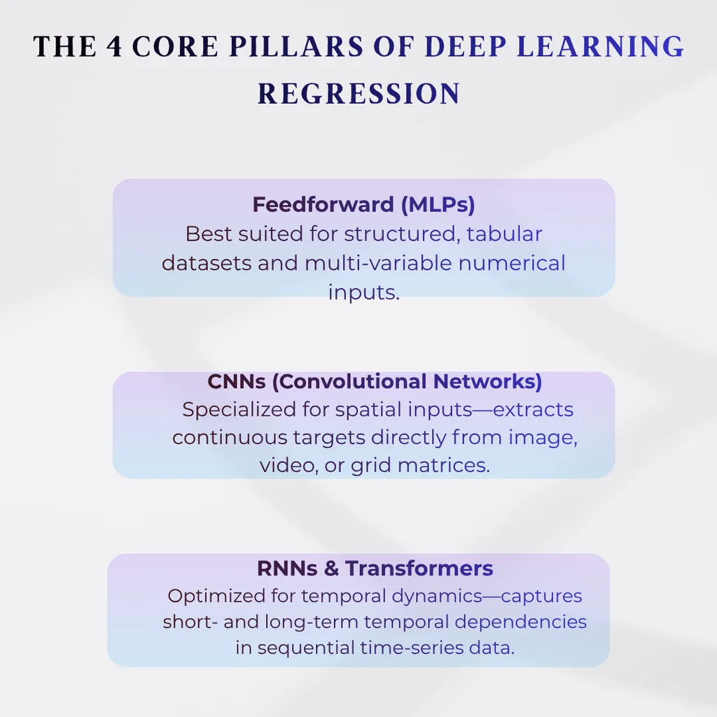
Deep learning eliminates the need for predefined functional forms by using multi-layered artificial neural networks as universal function approximators. These architectures autonomously capture non-linear, multi-factorial relationships directly from raw inputs.
The primary building blocks of deep learning regression include:
- Architectures:
- Feedforward Neural Networks (Multilayer Perceptrons): Ideal for structured tabular data.
- Convolutional Neural Networks (CNNs): Applied when continuous targets depend on spatial inputs (e.g., predicting continuous property values from satellite or house imagery).
- Recurrent Architectures & Transformers (LSTMs, GRUs, Temporal Fusion Transformers): Optimized for sequential time-series forecasting.
- Target Loss Functions:
- Mean Squared Error (MSE): Heavily penalizes large errors; sensitive to outliers.
- Mean Absolute Error (MAE): Penalizes errors linearly, offering robust performance against noisy targets.
- Huber Loss: Combines the smooth convergence of MSE near zero with the outlier resistance of MAE.
- Quantile Loss: Predicts specific percentiles to output prediction intervals rather than single-point estimates.
- Feature Representation: Neural networks automatically extract hierarchical representations, reducing reliance on manual feature interaction engineering. Basic preprocessing—such as z-score standardization, min-max scaling, and dense embeddings for high-cardinality categorical features—remains mandatory to ensure gradient stability.
Deep Learning vs. Traditional Regression
| Dimension | Traditional Regression (OLS, Ridge, Lasso) | Deep Learning Regression |
| Relationship Modeling | Linear or explicitly specified polynomials | Arbitrary non-linear and high-order interactions |
| Data Requirements | Small to moderate datasets | Large volumes of labeled data |
| Interpretability | High (direct coefficient interpretation) | Low (“black-box” model representations) |
| Computational Cost | Minimal CPU overhead | High GPU/TPU compute requirements |
| Data Types | Structured, tabular data | Tabular, sequential, image, and multi-modal data |
Industry Applications
- Quantitative Finance: Generating continuous signals for algorithmic trading, volatility estimation, and macroeconomic trend forecasting.
- Precision Healthcare: Estimating continuous clinical markers, patient recovery durations, and tumor volumetric growth directly from multi-modal EHRs and bioimaging.
- Grid & Energy Management: Predicting high-frequency smart grid load spikes and renewable generation capacity based on environmental sensor telemetry.
- Supply Chain Logistics: Modeling dynamic consumer demand across millions of SKUs with multi-horizon time-series transformers to automate replenishment.
Technical Challenges and Bottlenecks
- Data Hunger: Neural networks fail to generalize without sufficient data volume, leading to poor performance compared to gradient-boosted trees (e.g., XGBoost, LightGBM) on small tabular datasets.
- Interpretability Deficits: In high-stakes regulatory environments (e.g., credit scoring, clinical diagnosis), the unexplainable nature of hidden layer weights necessitates post-hoc interpretability frameworks like SHAP (SHapley Additive exPlanations) or Integrated Gradients.
- Overfitting Risks: High parameter counts allow deep models to memorize label noise. Preventing generalization failure requires explicit regularization, such as weight decay ($L_1/L_2$), dropout layers, early stopping, and batch normalization.
Future Directions:
Despite the challenges, the field of deep learning for regression continues to evolve rapidly, driven by advances in hardware, algorithms, and data availability. Some promising directions for future research and development include:
- Transfer Learning: Transfer learning techniques, where pre-trained deep learning models are fine-tuned on specific regression tasks, can help mitigate the data scarcity problem and accelerate model development.
- Explainable AI: Research into explainable AI aims to enhance the transparency and interpretability of deep learning models, enabling stakeholders to understand and trust the model predictions.
- Bayesian Deep Learning: Bayesian deep learning methods integrate probabilistic frameworks with deep neural networks, enabling uncertainty quantification and robustness to noisy or incomplete data.
Read more blog : How AI and Machine Learning Are Changing Stock Market Trading in 2026?

ConclusionDeep learning holds tremendous potential for regression analysis, offering a flexible and powerful framework for modeling complex relationships in data. By leveraging deep neural networks, researchers and practitioners can tackle a diverse array of regression tasks across industries, from finance and healthcare to energy and retail. While challenges remain, ongoing research and innovation are poised to further enhance the efficacy and applicability of deep learning for regression in the years to come. As we continue to unlock the mysteries of deep learning, the possibilities for regression analysis are boundless, paving the way for transformative advancements in predictive modeling and data-driven decision-making.If you’re interested in staying updated with the latest insights and trends in artificial intelligence, deep learning, and data science, I invite you to connect with me on LinkedIn. Let’s continue the conversation and explore the exciting opportunities in these cutting-edge fields together!
Frequently Ask Question :
When should I choose deep learning over gradient boosting (like XGBoost or LightGBM) for regression?
Deep learning excels when working with unstructured or multi-modal inputs (e.g., images, text, and sensor feeds combined with numbers) or highly dynamic, large-scale sequential data. For standard, tabular, structured datasets of moderate size, gradient-boosted decision trees typically train faster, require less tuning, and often yield equal or superior predictive accuracy.
What is the difference between Mean Squared Error (MSE) and Huber Loss in regression training?
MSE squares the differences between predicted and actual values, which disproportionately penalizes large errors and makes models highly sensitive to extreme outliers. Huber Loss functions quadratically when errors are small (ensuring smooth gradient descent near the minimum) but transitions to linear penalties for larger errors, providing a balanced trade-off between convergence stability and outlier robustness.
Why is feature scaling essential before training a neural network for continuous targets?
Neural network weights update using gradient-based optimization algorithms. If input features operate on widely divergent scales, gradients can oscillate, explode, or vanish, slowing down or entirely preventing model convergence. Techniques like z-score standardization ($Z = \frac{x – \mu}{\sigma}$) or min-max normalization ensure balanced gradient updates across all network layers.
Can deep learning output a prediction interval instead of a single point estimate?
Yes. By training models using Quantile Loss (pinball loss) across designated percentiles (such as the 10th, 50th, and 90th percentiles), or by applying Bayesian deep learning techniques like Monte Carlo Dropout, neural networks can estimate confidence bands and quantify prediction uncertainty alongside the expected value.
